Difference between revisions of "April 12, 2019"
| (23 intermediate revisions by the same user not shown) | |||
| Line 4: | Line 4: | ||
Alex and I have settled on an ideal way to deal with the photometric redshift uncertainties on the RedMaPPer (RM) cluster data. The plan is to divide everything into fairly small redshift slices, corresponding to around 30 Mpc. For each slice, I'll make a projected number density map with the CMASS galaxies. (They have very low redshift uncertainties so they are essentially guaranteed to truly exist in that slice.) For every RM cluster, the catalog provides not only the calculated mean photo-z but also the probability distribution of photo-z. Therefore, for each redshift slice, I'll take every RedMaPPer cluster that has any probability of being in that slice (including those whose mean photo-z falls in another slice), and run these through COOP to get the orientation vector for each cluster. For example, if a cluster's photo-z probability extends over the z=.2 to .21 slice, the z=.21 to .22 slice, and the z=.22 to .23 slice, I will run this cluster with the orientation map for each of those bins and get 3 orientations out. Finally, I'll write my own stacking code which, for a single redshift slice of 30Mpc, stacks all the clusters that could possibly exist somewhere in that slice, orients them with the imported COOP orientations, and weights each cluster by the probability that it exists in that slice. (That probability is the area under the photo-z curve within that slice). With this method, we can do oriented stacks for reasonably small redshift slices and fully account for the uncertainties in the photometric redshifts of clusters. | Alex and I have settled on an ideal way to deal with the photometric redshift uncertainties on the RedMaPPer (RM) cluster data. The plan is to divide everything into fairly small redshift slices, corresponding to around 30 Mpc. For each slice, I'll make a projected number density map with the CMASS galaxies. (They have very low redshift uncertainties so they are essentially guaranteed to truly exist in that slice.) For every RM cluster, the catalog provides not only the calculated mean photo-z but also the probability distribution of photo-z. Therefore, for each redshift slice, I'll take every RedMaPPer cluster that has any probability of being in that slice (including those whose mean photo-z falls in another slice), and run these through COOP to get the orientation vector for each cluster. For example, if a cluster's photo-z probability extends over the z=.2 to .21 slice, the z=.21 to .22 slice, and the z=.22 to .23 slice, I will run this cluster with the orientation map for each of those bins and get 3 orientations out. Finally, I'll write my own stacking code which, for a single redshift slice of 30Mpc, stacks all the clusters that could possibly exist somewhere in that slice, orients them with the imported COOP orientations, and weights each cluster by the probability that it exists in that slice. (That probability is the area under the photo-z curve within that slice). With this method, we can do oriented stacks for reasonably small redshift slices and fully account for the uncertainties in the photometric redshifts of clusters. | ||
| − | However, re-writing and re-organizing my code to do this will be a long enough task that I won't be able to do it by the end of 1501. For | + | However, re-writing and re-organizing my code to do this will be a long enough task that I probably won't be able to do it by the end of 1501. For now, I'll simply take slices of 100 comoving Mpc, make number density maps with all the CMASS galaxies in those slices, and assume that the RM clusters' photo-zs are accurate. |
| − | + | == Numbers of Objects == | |
| + | For 100 Mpc slices, these are the amount of RedMaPPer (RM) clusters and CMASS galaxies in each slice which are also within the ACT region: | ||
| − | + | [[File:Cls and gals histogram v3.png]] | |
| − | + | [[File:Zbin histogram.png]] | |
| − | |||
| − | + | == Example Plots of CMASS Sample == | |
| − | |||
| − | |||
| − | |||
| − | |||
| − | |||
| − | |||
| − | |||
| − | |||
| − | |||
| − | |||
| − | |||
| − | |||
| − | |||
| − | |||
| − | |||
| − | |||
| − | |||
| − | |||
| − | |||
| − | |||
| − | |||
| − | |||
| − | |||
| − | |||
| − | |||
| − | |||
| − | |||
| − | |||
| − | |||
| − | |||
| − | |||
| − | |||
| − | |||
| − | |||
| − | |||
| − | |||
| − | |||
| − | |||
| − | |||
| − | |||
| − | |||
| − | |||
| − | |||
| − | |||
| − | |||
| − | |||
| − | |||
| − | |||
| − | |||
| − | |||
| − | |||
| − | |||
| − | + | As you can see above, the most populated bin in the DES sample is at z~0.57. As an example, I've plotted the galaxies and clusters for this redshift slice. I'm including more sky coverage for the galaxies because I want them to cover the edge clusters. | |
| − | + | [[File:Zpt57 cls and gals v3.png]] | |
| − | + | Next, I make a Healpix Nside=2048 map where I put a '1' down in every pixel where there's a galaxy from the CMASS sample. Then I smooth this map with a 25' Gaussian beam. Here is the resulting smoothed number-density map for this redshift slice. | |
| − | + | [[File:CMASS z pt556topt588 smooth25arcminv2.png]] | |
| − | + | To my eye, this looks like the galaxies are showing real large-scale-structure, but I think we might need to be careful given what the entire CMASS sample looks like: | |
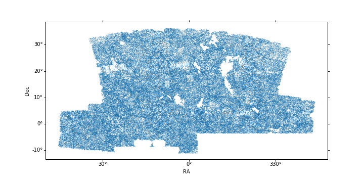
| − | + | [[File:Full sample plot.png]] | |
| − | + | In some areas where the coverage isn't as dense, it looks like there are lines of galaxies. Maybe the survey scanned in that direction; I'll have to look more into that. I think the effect of this should be cancelled out when we subtract a stack on random points, but it's something to keep in mind. | |
| − | + | == Matching with Simulations == | |
| − | + | To match Peak Patch halos with the DES clusters, I'm taking the top n most massive clusters from the Peak Patch run for each redshift slice, where n is the number of DES clusters in that redshift slice. | |
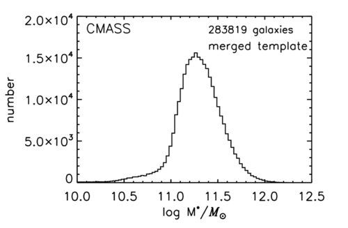
| − | + | The BOSS CMASS sample is chosen to have approximately constant mass, as shown in this histogram taken from Maraston et al 2013 ([https://arxiv.org/pdf/1207.6114.pdf]). | |
| − | + | [[File:CMASS masses.png|500px]] | |
| − | |||
| − | |||
| − | |||
| − | |||
| − | |||
| − | |||
| − | |||
| − | |||
| − | |||
| − | |||
| − | |||
| − | |||
| − | |||
| − | + | Alex had suggested that, rather than populating the simulation halos with central and satellite galaxies and matching those to the CMASS stellar mass, it might be better to find an estimate for the CMASS halo mass and use Peak Patch halos with that mass. According to this study ([https://arxiv.org/pdf/1811.04934.pdf]), the log halo mass at the CMASS average log stellar mass of 11.4 M_sun is 12.79 M_sun. Therefore I am finding Peak patch halos around that mass, and matching the number in each redshift slice to the numbers in the CMASS sample. | |
Latest revision as of 18:01, 24 April 2019
April Updates
Status of the Project
Alex and I have settled on an ideal way to deal with the photometric redshift uncertainties on the RedMaPPer (RM) cluster data. The plan is to divide everything into fairly small redshift slices, corresponding to around 30 Mpc. For each slice, I'll make a projected number density map with the CMASS galaxies. (They have very low redshift uncertainties so they are essentially guaranteed to truly exist in that slice.) For every RM cluster, the catalog provides not only the calculated mean photo-z but also the probability distribution of photo-z. Therefore, for each redshift slice, I'll take every RedMaPPer cluster that has any probability of being in that slice (including those whose mean photo-z falls in another slice), and run these through COOP to get the orientation vector for each cluster. For example, if a cluster's photo-z probability extends over the z=.2 to .21 slice, the z=.21 to .22 slice, and the z=.22 to .23 slice, I will run this cluster with the orientation map for each of those bins and get 3 orientations out. Finally, I'll write my own stacking code which, for a single redshift slice of 30Mpc, stacks all the clusters that could possibly exist somewhere in that slice, orients them with the imported COOP orientations, and weights each cluster by the probability that it exists in that slice. (That probability is the area under the photo-z curve within that slice). With this method, we can do oriented stacks for reasonably small redshift slices and fully account for the uncertainties in the photometric redshifts of clusters.
However, re-writing and re-organizing my code to do this will be a long enough task that I probably won't be able to do it by the end of 1501. For now, I'll simply take slices of 100 comoving Mpc, make number density maps with all the CMASS galaxies in those slices, and assume that the RM clusters' photo-zs are accurate.
Numbers of Objects
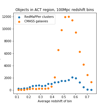
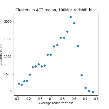
For 100 Mpc slices, these are the amount of RedMaPPer (RM) clusters and CMASS galaxies in each slice which are also within the ACT region:
Example Plots of CMASS Sample
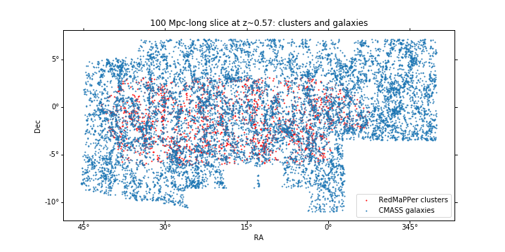
As you can see above, the most populated bin in the DES sample is at z~0.57. As an example, I've plotted the galaxies and clusters for this redshift slice. I'm including more sky coverage for the galaxies because I want them to cover the edge clusters.
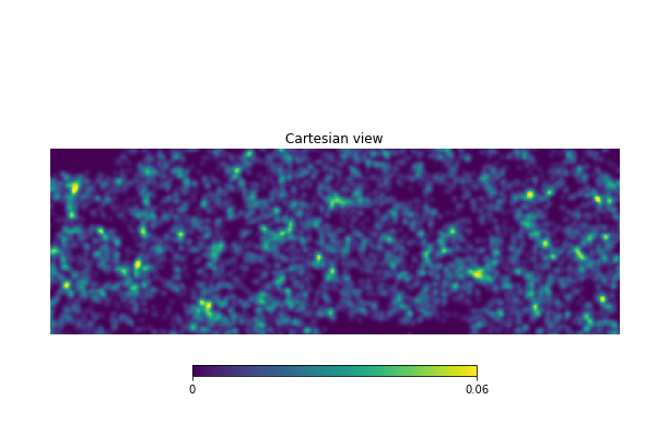
Next, I make a Healpix Nside=2048 map where I put a '1' down in every pixel where there's a galaxy from the CMASS sample. Then I smooth this map with a 25' Gaussian beam. Here is the resulting smoothed number-density map for this redshift slice.
To my eye, this looks like the galaxies are showing real large-scale-structure, but I think we might need to be careful given what the entire CMASS sample looks like:
In some areas where the coverage isn't as dense, it looks like there are lines of galaxies. Maybe the survey scanned in that direction; I'll have to look more into that. I think the effect of this should be cancelled out when we subtract a stack on random points, but it's something to keep in mind.
Matching with Simulations
To match Peak Patch halos with the DES clusters, I'm taking the top n most massive clusters from the Peak Patch run for each redshift slice, where n is the number of DES clusters in that redshift slice.
The BOSS CMASS sample is chosen to have approximately constant mass, as shown in this histogram taken from Maraston et al 2013 ([1]).
Alex had suggested that, rather than populating the simulation halos with central and satellite galaxies and matching those to the CMASS stellar mass, it might be better to find an estimate for the CMASS halo mass and use Peak Patch halos with that mass. According to this study ([2]), the log halo mass at the CMASS average log stellar mass of 11.4 M_sun is 12.79 M_sun. Therefore I am finding Peak patch halos around that mass, and matching the number in each redshift slice to the numbers in the CMASS sample.
