Oct 17, 2018 - Lensing the CIB
CIB Lensing of Individual Shells and Analysis
Here is what I was able to do. The difference between the unlensed and lensed maps in this post are not quite clear. For a better comparison, the images can be opened in two separate tabs (to full screen): one for the unlensed and one for the lensed. Moving between the tabs, the difference should be evident.
1. Lens the 23 CIB maps with the 23 kappa maps, creating a [math]\displaystyle{ cib_i^{lensed} }[/math] and a [math]\displaystyle{ cib_i^{unlensed} }[/math] set of 23 maps.
  I only used the field maps for both the kappa and the CIB maps. There were only 16 maps for the field (from z = 0 to z = 3.2).
  Used the bash script Remi left. The following is the part of my script that did the lensing.
  It turned out this was where I made a mistake before and got such high values for the fractional difference between the lensed
  and unlensed maps. I had been lensing a CIB map with the kappa map of the same range of z which does not make sense since a CIB shell
  will only be lensed by the kappa before it. For example, CIB_z_1.0_1.2 has to be lensed by Kappa_z_0.8_1.0_zsource_0.9 but I was
  lensing it with Kappa_z_1.0_1.2_zsource_1.1.
     for i in seq 0.2 0.2 3.2;
     do
      echo "-----------$i----------"
      zmid=`awk "BEGIN {print $i-0.1}"`
      zfield=`awk "BEGIN {print $i+0.2}"`
      echo "$zmid"
      echo "$zfield"
      python lens.py ../jason_cib_lensing/maps/kappa/field/kappa_field_nside2048_zmin0.0_zmax${i}_zsource${zmid}_kap.fits
      ../jason_cib_lensing/maps/cib/field/2048/unlensed_maps/cib_field_nside2048_zmin${i}_zmax${zfield}_cib.fits
      ../jason_cib_lensing/maps/lensed/phi/run2/kap_zmax${i}_phi_field.fits
      ../jason_cib_lensing/maps/lensed/field/run2/cib_field_nside2048_zmin${i}_zmax${zfield}_cib_lensed.fits -np 40
2. Plot cartview "zoom ins" of a few cib maps, lensed and unlensed, to make sure the lensing makes sense.
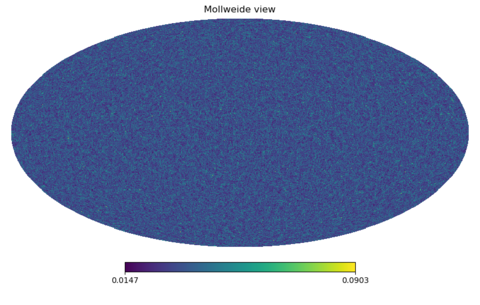
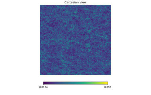
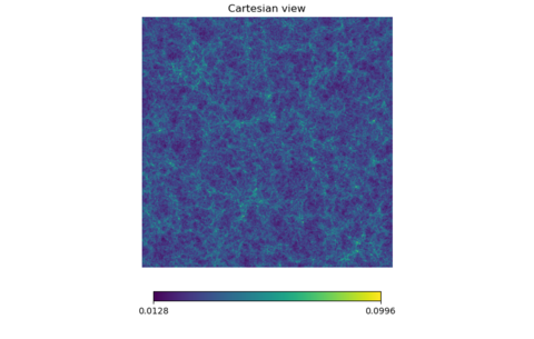
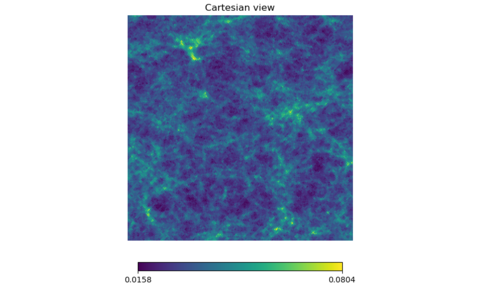
  I tried this out for z = 1.0 to 1.2 and z = 2.0 to 2.2, the whole map and some cartviews. The scales at the bottom were synchronized between
  lensed and unlensed maps.

   z = 1.0 to 1.2
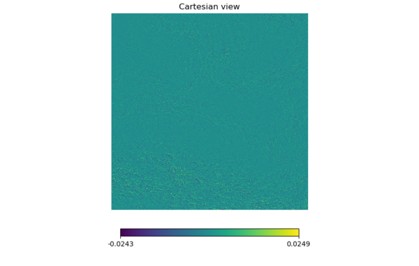
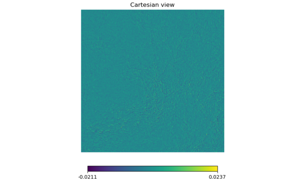
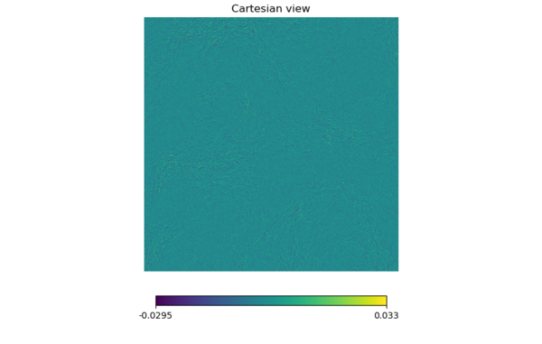
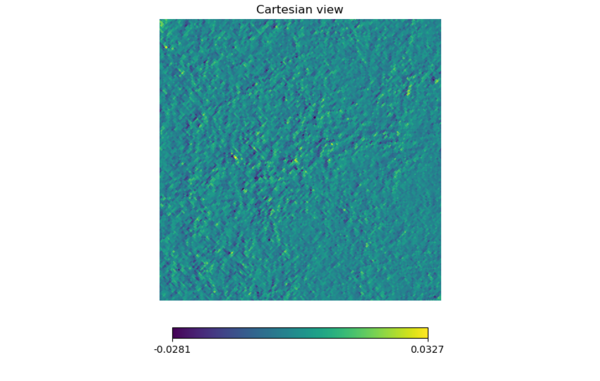
  There isn't a clear difference between the two maps so I subtracted the lensed map from the unlensed (linearly) and made a map out of it.
  I will refer to these as 'difference maps.' (It may be different from the difference maps mentioned in the last meeting.)
Now there is a difference for sure.
Again, the two maps look virtually the same and these are difficult to differentiate even with blinking.
This looks better.
The same goes for these maps even though the range is smaller.
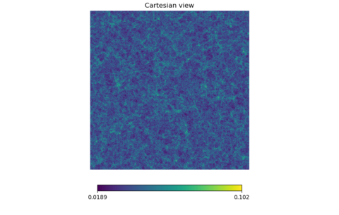
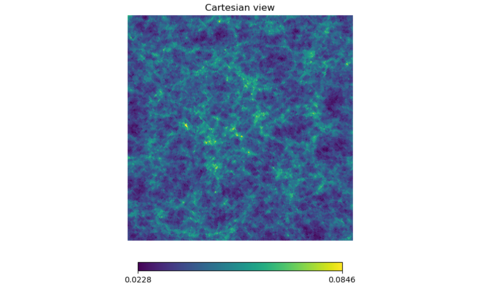
When the maps are zoomed into 5º patches, the two maps certainly display a difference even though details are blurred due to the resolution.
z = 2.0 to 2.2
It is hard to tell these two apart from each other as well but note that the scale is almost two times the scale for z = 1.0 to 1.2.
These two maps seem much different from each other compared to the 35º~40º for z = 1.0 to 1.2.
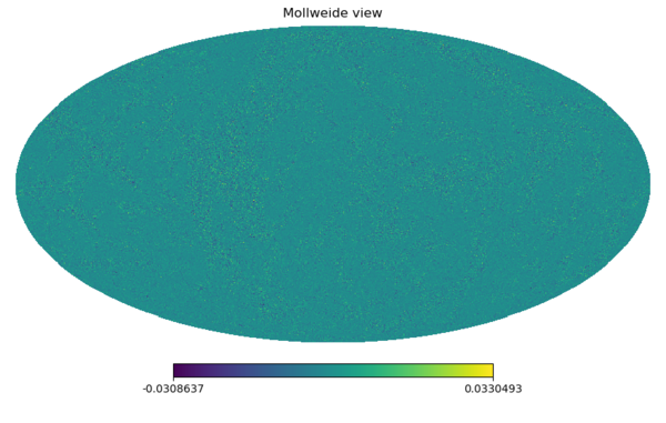
This map displays a huge amount of difference compared to other difference maps. It may be part of the reason why the scale for the total maps are larger compared to z = 1.0 to 1.2.
3. Add these 23 maps together to get a [math]\displaystyle{ cib_{total}^{lensed} = \sum_i cib_i^{lensed} }[/math] , and a [math]\displaystyle{ cib_{total}^{unlensed} = \sum_i cib_i^{unlensed} }[/math].
  Used a python script to add the maps up (with help from George). I also added CIB_z_0.0_0.2 which is the same before and after lensing. The script goes:

  import healpy as hp
  import glob
  import sys
  nside_f = 2048
  filelist = sorted(glob.glob('./*fit*'))
  map_f = 0
  for i in range(len(filelist)):
      print "adding map = ", filelist[i]
      map_i = hp.read_map(filelist[i])
      print(map_i)
      map_f = map_f + map_i
      print(map_f)
  hp.write_map("added_map.fits", map_f)
4. Plot these, and also take their power spectra and plot those just like you did for the CMB lensing (getting a Δ[math]\displaystyle{ C_l/C_l }[/math] too).
  Note: The y-axis for the [math]\displaystyle{ C_l }[/math] spectra were not scaled. It has to be multiplied by (presumably) a factor of [math]\displaystyle{ 10^6 }[/math]
  or [math]\displaystyle{ 10^{12} }[/math] depending on the unit of measurement.
Total Maps
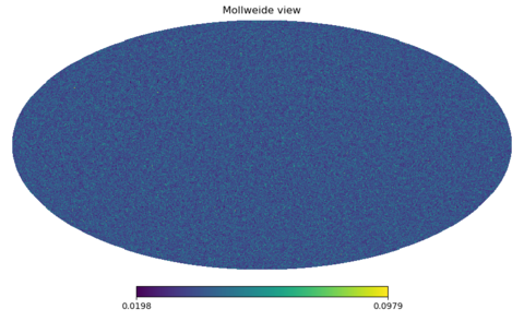
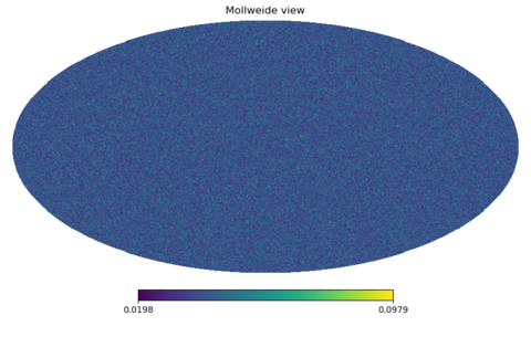
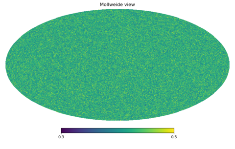
The scales have become bigger but there isn't an obvious difference.
Now the scales are about 2~3 times the range of the difference maps given above with individual shells. (z = 1.0 to 1.2 and z = 2.0 to 2.2 must contribute a lot.)
Power Spectrum
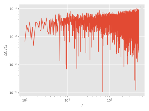
It is hard to distinguish the two curves even when the scales are set differently for a better view. The vertical distance between the unlensed/lensed spectra and the difference decreases as [math]\displaystyle{ l }[/math] becomes larger, implying that the fractional difference will increase with [math]\displaystyle{ l }[/math].
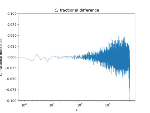
Fractional Difference (Given by [math]\displaystyle{ (cib_{lensed} - cib_{unlensed})/cib_{unlensed} }[/math])
  The amplitude of the fractional difference between the total unlensed and lensed CIB is shown to be around -5% to 5%.
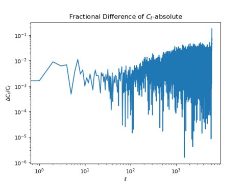
  When the scale is set to log, it is evident that the fractional difference increases as [math]\displaystyle{  l  }[/math] increases on a logarithmic scale (smaller
  patches of sky).
The absolute value of the fractional difference was plotted in order to compare with Remi's graph. The two display similar tendencies but Remi's fractional difference is larger overall. This may be because Remi was using more maps (more slices than me perhaps?).
5. The power spectra of each of the 23 slices lensed and unlensed may be taken separately to see whats going on.
I tried this out for the range of 'z' I used for the maps above.
z = 1.0 to 1.2
Power Spectrum
Again, there isn't lot to be said comparing the two. The maximum of the [math]\displaystyle{ C_l }[/math] spectra are 10 ~ 50 times smaller compared to the [math]\displaystyle{ C_l }[/math] spectra of the total maps. This makes sense.
Fractional Difference
However, the fractional difference seem quite similar to the added maps' fractional difference. This may imply that a lot of the effects of CIB lensing are canceled out when the shells are added up. (The fractional difference does have a bigger amplitude when the maps are added up,)
z = 2.0 to 2.2
Power Spectrum
Fractional Difference
Here, the amplitude of the fractional difference is even larger than before, maybe even larger than the added maps' fractional difference. This further strengthens the idea that CIB lensing is canceled out when shells are added.
Summary I have lensed CIB maps from z = 0 to z = 3.2, took a look at the maps and zoomed in for a range of z = 1.0 to 1.2 and 2.0 to 2.2. The maps didn't show much of a difference when looking at patches of 20º~ 30º but the difference was noticeable for patches of 5º. Difference maps were also plotted to demonstrate the effect of lensing. Afterwords, the power spectrum and fractional difference were plotted for the added maps. The power spectrum did not display much of a difference, but the fractional difference showed the effect of lensing on the CIB to be around 2~4%. Finally, the power spectrum and fractional difference of two shells were investigated. The spectra itself were at least 10 times smaller compared to the added maps, but the fractional difference were of the same order of magnitude, implying that the fractional differences do not add up.
