April 21, 2019 - The origin of the excess kurtosis (revised)

I have looked into why the filtered kurtosis values of the Gaussianized CIB map start to rise at an ell of around 4000, away from 0. I ran the top-hat filters through maps of NSIDE = 1024, 2048, and 4096. I also tried smoothing out the edges of the top-hat filters for NSIDE = 2048.

1. NSIDE effect

i) NSIDE = 1024

ii) NSIDE = 2048

iii) NSIDE = 4096

It seems almost certain that the excess kurtosis is an NSIDE artefact, as the rise starts at roughly ell = 2/3*l_max for each case and the amount of increase is essentially the same as well.

2. Top-hat filters edge effect

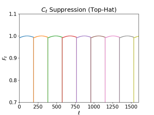
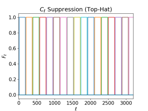
- how the edge-smoothed filters look for NSIDE = 2048 (used a cosine function)

i) sharp edges

ii) smooth edges

The edges of the top-hat filters don't seem to affect results much; I could try defining filters with an exponential function rather than a cosine function so that F_l decreases more dramatically near the edges, but I don't expect a lot of difference.

Conclusion

It seems that I should use NSIDE = 4096 maps for the kurtosis at least.

REVISION

I created another set of smoothed top-hat filters using Pavel's apodization method - https://mocks.cita.utoronto.ca/index.php/Jan_22,_2019_-_Using_wrong_map:_Skewness_and_Kurtosis,_top_hat_filter_with_blunt_edges.

I simply replaced [math]\displaystyle{ \frac{1}{2}\left(1 + \sin \frac{\pi (x - x_\mathrm{edge})}{2 \Delta}\right) . }[/math] within [math]\displaystyle{ [-\Delta, \Delta] }[/math] near the edges of the top-hats (+- 10 for a bandwidth of 192).

i) F_l plots

These filters look different from Pavel's in https://mocks.cita.utoronto.ca/index.php/Jan_23,_2019_-_Comparison_of_mine_and_Jason%27s_filters , and I do not quite understand why the top-hat filter for the last bandwidth isn't defined, but I thought it should do for now, just to see the trends.

ii) Top-hat filtered variance, skewness, kurtosis

As before, these plots show little difference from the ones above with different edges.