July 18th, 2019 - CIB Total Maps Analysis
In this post, I am providing some analysis on some of the effects caused by splitting the shells, filtering them and adding the statistics back together, and other more mysterious effects.
Histograms
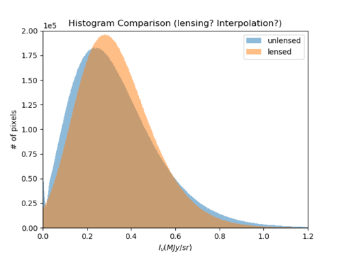
Below are the histograms before and after lensing, which contains the lensing, interpolation, and other additional effects.
What is puzzling is that the lensing itself does not cause the original CIB histogram to change so much; when I looked at smoothed CIB and null lensed CIB histograms, they were practically the same as the "lensed" histogram given above.
Something unexpected is that this discrepancy between the two histograms does not affect the n-point functions (at least for n = 2, 3 the change caused is less than 0.1%).
Cumulative Analysis
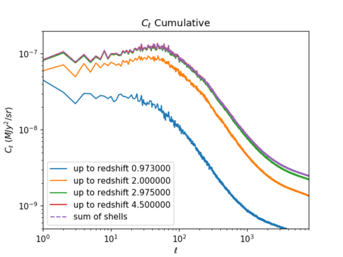
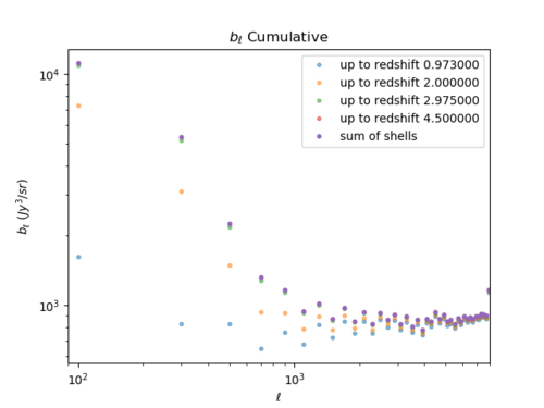
Below are plots of the contribution to the power spectrum and bispectrum by redshift range.
- Power Spectra, Bispectra
The power spectrum seems to come primarily from redshift 1 to 3, while this is not the case for the reduced bispectrum. [math]\displaystyle{ b_{\ell} }[/math] mostly comes from redshift 0 to 1 (especially for high [math]\displaystyle{ \ell }[/math].
Contribution of Closest 100 Mpcs to the Bispectrum
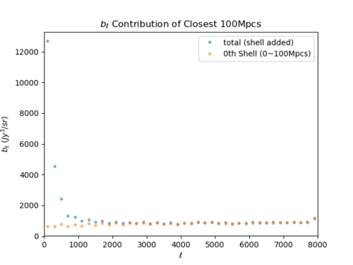
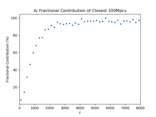
Below are plots showing the contribution of the first 100 Mpcs of the CIB to the reduced bispectrum.
The contribution rapidly increases to over 90% by [math]\displaystyle{ \ell \approx 2000 }[/math]; as the 0th shell is not lensed, the lensing cannot change the bispectrum by more than a few percent (at most) when [math]\displaystyle{ \ell \gt 2000 }[/math]. (Is this acceptable?)
Total Map Filtered vs. Shell Filtered Then Added
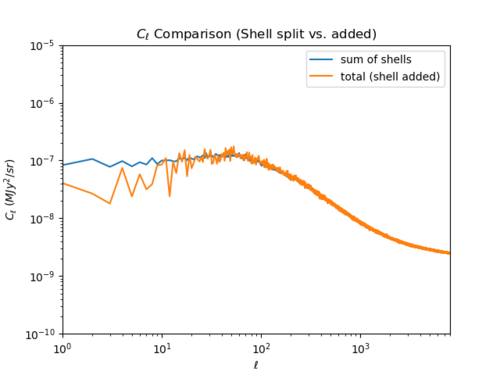
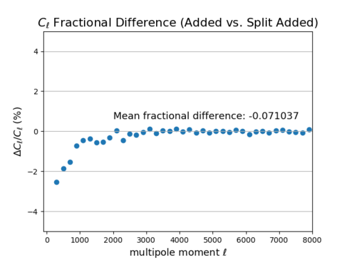
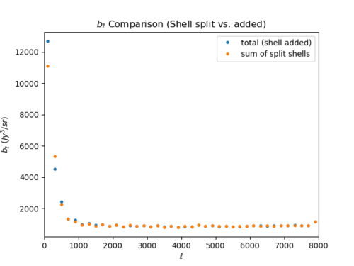
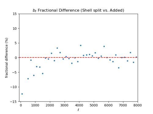
The plots here show the difference between the total CIB statistics and added shell statistics (by filtering each shell, then adding up each shell's statistics) at the power spectrum and bispectrum levels. For both [math]\displaystyle{ C_{\ell} }[/math] and [math]\displaystyle{ b_{\ell} }[/math], correlation between the shells seem to exist at [math]\displaystyle{ \ell \lt 2000 }[/math] as the shell statistics added up are smaller than the total statistics (I apologize for the confusing colors between the [math]\displaystyle{ C_{\ell} }[/math] and [math]\displaystyle{ b_{\ell} }[/math] for the left plots.) There seems to be more correlation between the shells for [math]\displaystyle{ b_{\ell} }[/math] compared to [math]\displaystyle{ C_{\ell} }[/math].
- Power Spectra
- Bispectra
