June 29th, 2020 - CIB Lensing: Lenspix - Deflection

Because we were seeing negative pixels in lensed CIB maps produced by 'lenspix,' I tried simulating the lensing by deflecting the galaxies by their corresponding deflection angles calculated using the [math]\displaystyle{  \kappa  }[/math] maps. 
Since 'lenspix' produces [math]\displaystyle{  \psi_lm  }[/math] maps (and I checked that their values are legitimate), I used equations from the appendix of Lewis (2005), https://arxiv.org/pdf/astro-ph/0502469.pdf as a reference to calculate the deflection angles. 

There, it is mentioned that 'the lensed temperature at a position [math]\displaystyle{  (\theta, \phi)  }[/math] is given by the unlensed temperature at position [math]\displaystyle{  (\theta', \phi + \Delta \phi)  }[/math], where:

[math]\displaystyle{  \cos \theta' = \cos d \cos \theta - \sin d \sin \theta \cos \alpha  }[/math] & [math]\displaystyle{  \sin \Delta \phi = \frac{\sin\alpha \sin d}{\sin \theta'}  }[/math], and the deflection vector is [math]\displaystyle{  \nabla \psi = d_{\theta} \mathbf{e_{\theta}} + d_{\phi} \mathbf{e_{\phi}} = d \cos \alpha \mathbf{e_{\theta}} + d \sin \alpha \mathbf{e_{\phi}}  }[/math]. ( Lewis ) - It seems I should be able to be derive this from the cosine law on the sphere, but I wasn't able to yet.

However, using the diagram below and spherical trignometry, I got: 
(Pythagorean theorem) [math]\displaystyle{  \cos d = \cos \Delta \phi \cos (\theta' - \theta)  }[/math],  [math]\displaystyle{  \theta = \theta' - [\cos^{-1} \frac{\cos\theta}{\cos \Delta \phi}]  }[/math]
(Sine Law) [math]\displaystyle{  \frac{\sin \Delta \phi}{\sin \alpha} = \frac{\sin d}{\sin 90}  }[/math],  [math]\displaystyle{   \Delta \phi = [\sin^{-1} (\sin\alpha \sin d)]  }[/math] ( Right )

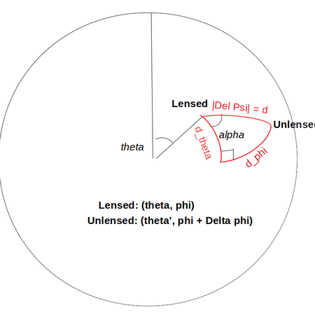
In the last case, I simply used [math]\displaystyle{  \theta' - \theta = d_{\theta}  }[/math] and [math]\displaystyle{  \Delta \phi = d_{\phi}  }[/math]. ( Euclidean )

I made maps for the three cases above - I will refer to them as 'Lewis', 'Right', and 'Euclidean (Approximation).' 
<Note> Since I could not preserve the signs (+, -) of the deflection directions for 'Lewis' and 'Right', I took the absolute values of the calculated angles and moved them in the same direction as for 'Euclidean.' 

3 versions of Deflected maps

The characteristics of the maps (unlensed, the 3 deflected maps, and 'lenspix' lensed) are as below. (I'll add the values for the 'Euclidean' deflected map as soon as possible)

Map Characteristics
	Unlensed	Deflected (Euclidean)	Deflected (Right)	Deflected (Lewis)	Lensed (Lenspix)
Max values (MJy/sr)	6.408424 (= 400 mJy)	6.408424	6.408424	6.408424	6.408424
Min values (MJy/sr)	0.000000	0.000000	0.000000	0.000000	-0.322438
# of pixels smaller than 0	0	0	0	0	1477969
Mean	0.3179518	0.3179518	0.3179518	0.3179518	0.3180850
Variance	0.0331789		0.0321213	0.0320472	0.0264728
Skewness	1.720313		1.740189	1.742209	1.776150
Kurtosis	23.366768		24.801155	24.912688	35.614250

For the deflected maps, we see that their variances are slightly smaller than the unlensed map, while their skewness' and kurtosis' are slightly larger. For the 'lenspix' lensed map, we see again a substantial decrease in the variance and increases in the mean, skewness and kurtosis (by a big amount). 

Histograms (Unlensed vs. Lenspix vs. Euclidean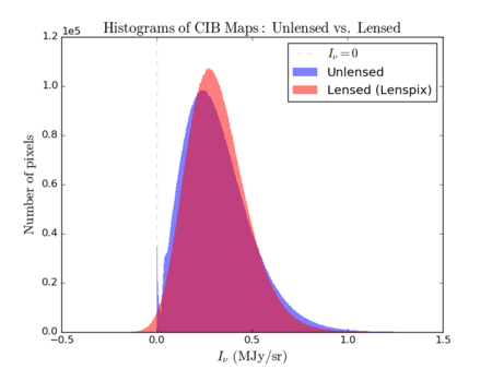
 

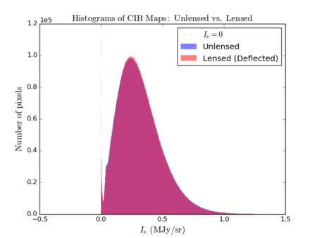
This is a comparison of the histograms - there is a slight difference (a tiny shift to the right) between the unlensed and (Euclidean) deflected histograms. As before, the lenspix-lensed map has negative pixels.  

Maps (lensed by total [math]\displaystyle{ \kappa }[/math], units are (MJy/sr))

Below are visualizations of the deflection in comparison to the unlensed and lenspix-lensed map. Order: Unlensed, Deflected, Lensed. Longitude range: [math]\displaystyle{  (0, 2\pi)  }[/math], Latitude range: [math]\displaystyle{  (-\frac{\pi}{2}, \frac{\pi}{2} )  }[/math]. 

Longitude [0, 1] Latitude [0, 1] (Euclidean, Right Triangle, Lewis Equation)

Longitude [264, 265] Latitude [-20, -19] (Euclidean, Right Triangle, Lewis Equation)

Longitude [220, 221] Latitude [60, 61] (Euclidean, Right Triangle, Lewis Equation)

Longitude [44, 45] Latitude [-80, -79] (Euclidean, Right Triangle, Lewis Equation)

For the low-latitude visualizations, we see that all 3 deflected maps simulate the galaxies/pixels moving quite well - at higher latitudes, especially -80 deg, we see that Lewis' equation definitely simulates the deflection better. 

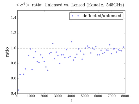
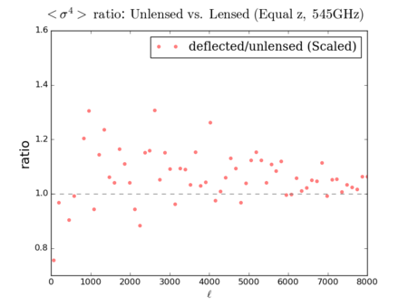
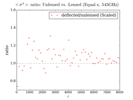
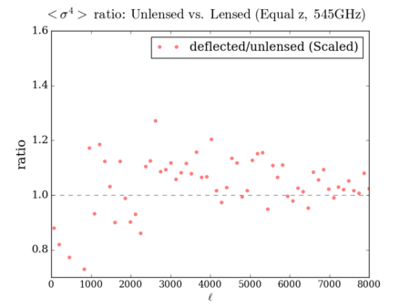
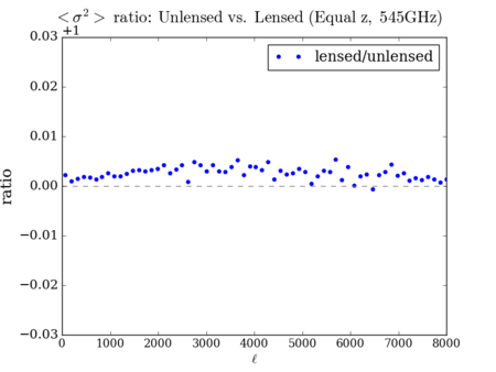
N-Point Statistics (3-point, 4-point, then 2-point)

Euclidean (Not scaled)
   

Euclidean (Scaled so the [math]\displaystyle{  C_{\ell}  }[/math] is unchanged) 3-point: divided by ([math]\displaystyle{  \lt \sigma^2\gt   }[/math] - ratio)^1.5, 4-point: divided by ([math]\displaystyle{  \lt \sigma^2\gt   }[/math] - ratio)^2
 

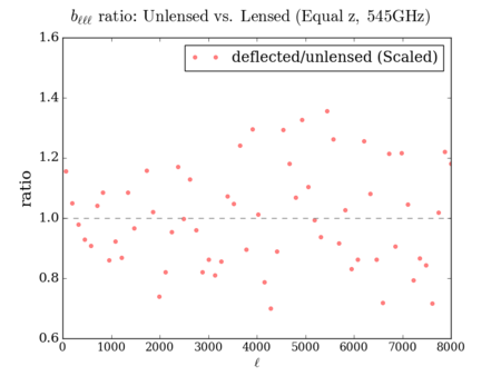
Right (Scaled so the [math]\displaystyle{  C_{\ell}  }[/math] is unchanged)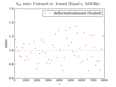
 

Lewis (Scaled so the [math]\displaystyle{  C_{\ell}  }[/math] is unchanged)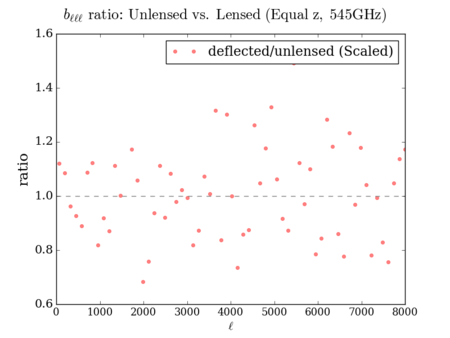
 

Lenspix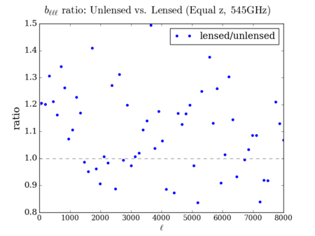
  

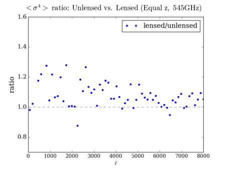
It is hard to see the difference between the three deflected versions - however, the scaled plots display some similarities with the 'lenspix' lensed map's at [math]\displaystyle{  \ell \gt  4000  }[/math] (especially for the 4-point). 

Summary
Through this exercise, we can see that the statistics given by 'lenspix' seem to make sense, even if this does not directly resolve the 'Negative Pixel' problem.