June 4th, 2019 - New Plots: Other Frequencies (217GHz, 353GHz)/Comparisons with Planck Data and Lacasa Model (Revised)

Below are some revised plots I made after Alex made some suggestions yesterday.

Reduced Bispectrum Plots

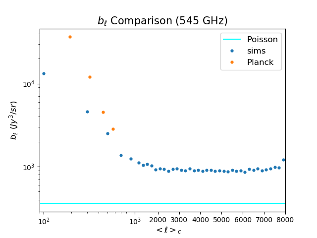
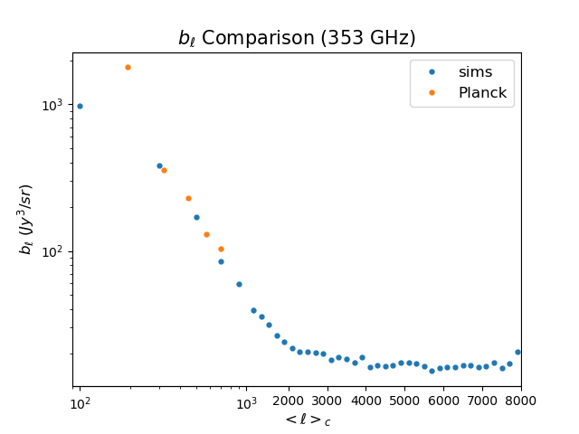
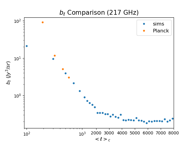
The left parts of the plots ([math]\displaystyle{ 0 \lt \ell \lt 1100 }[/math]) compare sims values to Planck values (log x-scale) while right parts go until [math]\displaystyle{ \ell \approx 8000 }[/math] on a linear x-scale.

I have not calculated the Poisson [math]\displaystyle{ b_{\ell} }[/math] values for 353GHz and 217GHz yet; George will be making new flux histograms for these this week.

- 545 GHz -

On the left, Planck's values are larger than sims values, but arguably follow a similar trend with [math]\displaystyle{ b_{\ell} }[/math] decreasing as [math]\displaystyle{ \ell }[/math] rises. On the right, as we've seen before, the expected [math]\displaystyle{ b_{\ell} }[/math] values calculated from the sims-filtered 3rd moment flatten out at higher [math]\displaystyle{ \ell }[/math] at about 2.5 times the Poisson value.

- 353 GHz -

For the 353GHz map, sims values match quite well with Planck values at low [math]\displaystyle{ \ell }[/math]. [math]\displaystyle{ b_{\ell} }[/math] flattens out at high [math]\displaystyle{ \ell }[/math] as before, but at a much lower value.

- 217 GHz -

For the 217GHz map, sims values match Planck values reasonably well, better than the 545GHz map at low [math]\displaystyle{ \ell }[/math]. Again, [math]\displaystyle{ b_{\ell} }[/math] flattens out at high [math]\displaystyle{ \ell }[/math], at an even lower value.

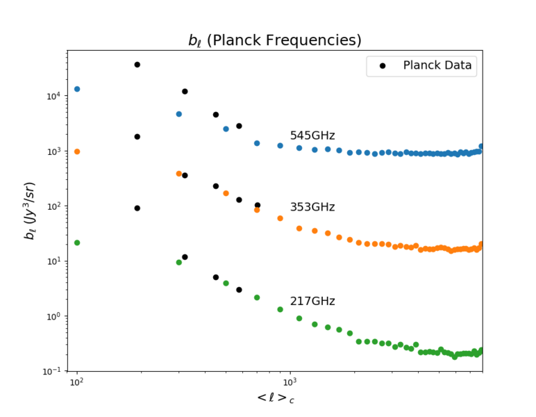
- All Planck Frequencies -

Comparison with Lacasa's clustering model

According to Lacasa et al. 2012 (Characterization of the non-Gaussianity of radio and IR point sources at CMB frequencies), a simple model for the clustering part of the bispectrum is [math]\displaystyle{ b_{{\ell_1} {\ell_2} {\ell_3}} \approx \alpha \sqrt{C_{\ell_1} C_{\ell_2} C_{\ell_3}} }[/math]. For equilateral configurations of [math]\displaystyle{ \ell }[/math], this simplifies to: [math]\displaystyle{ b_{\ell} \approx \alpha \sqrt{C_\ell ^3} }[/math] with [math]\displaystyle{ \alpha \approx 2.25 \times 10^{-3} }[/math]. Since Lacasa's model is relevant to just the clustering part, I subtracted out the Poisson [math]\displaystyle{ C_{\ell} }[/math] before calculating the [math]\displaystyle{ b_{\ell} }[/math], then took the sum of the clustering and Poisson [math]\displaystyle{ b_{\ell} }[/math] 's

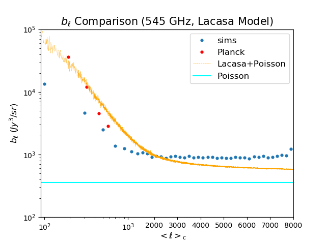
The modeled clustering part generally agrees with sims and Planck values at low [math]\displaystyle{ \ell }[/math]. On the right, Lacasa's model+Poisson values follow a similar trend to the sims values, although falling at a higher [math]\displaystyle{ \ell }[/math] but flattening at a lower amplitude of [math]\displaystyle{ b_{\ell} }[/math].

Filtering of tSZ

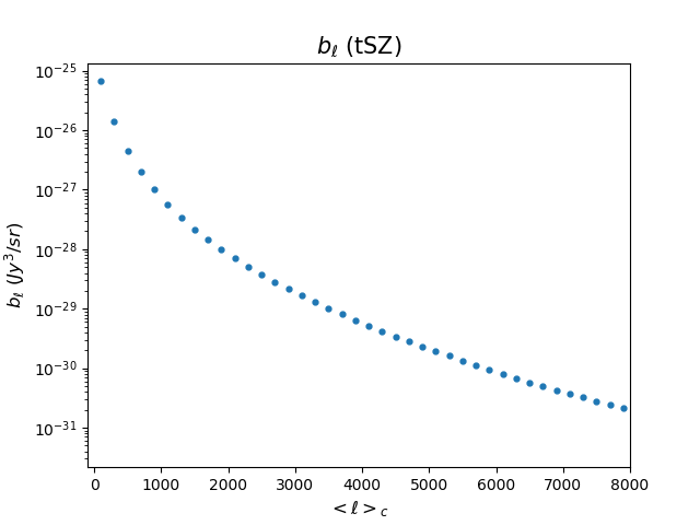
The following is the [math]\displaystyle{ b_{\ell} }[/math] of the tSZ map (log y-axis).

The values are generally much smaller than the CIB, though I am not sure whether I could directly compare these values with the CIB since they have different units (dimensionless for the tSZ, if I am not mistaken).