June 4th, 2019 - Reduced Bispectrum by Frequency (Fitted Plots)

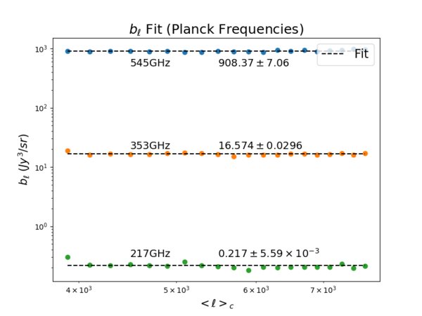
I made the plots below to find the relation between [math]\displaystyle{ b_{\ell} }[/math] at high [math]\displaystyle{ \ell }[/math] and the frequency, another consistency check suggested by Pavel. The standard deviations (errors) are calculated from the covariance matrices of the fits.

[math]\displaystyle{ b_{\ell} }[/math] Fits

I first fit the [math]\displaystyle{ b_{\ell} }[/math]'s to constant lines for each of the Planck frequencies (where the [math]\displaystyle{ b_{\ell} }[/math] values are listed) for [math]\displaystyle{ 3900 \le \ell \le 7700 }[/math]. The standard deviations are less than 1% for all frequencies, as expected from the flatness of the values at this range of [math]\displaystyle{ \ell }[/math].

Reduced Bispectrum vs. Frequency

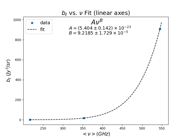
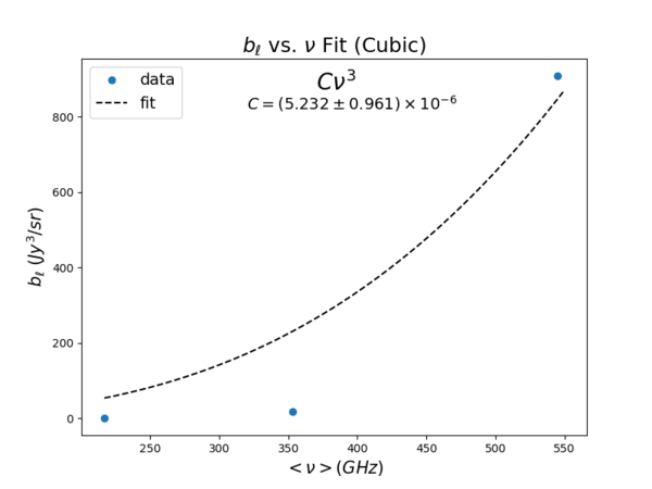
From the values of [math]\displaystyle{ b_{\ell} }[/math] obtained above, I tried fitting a general power law function [math]\displaystyle{ b_{\ell} = A\nu^B }[/math] and the function [math]\displaystyle{ b_{\ell} = C\nu^3 }[/math] to the [math]\displaystyle{ b_{\ell} }[/math] vs. [math]\displaystyle{ \nu }[/math] plot.

- Power Law [math]\displaystyle{ b_{\ell} = A\nu^B }[/math] -

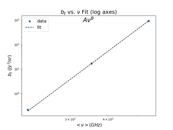
We first consider the plausibility of fitting a power law function by taking a look at the [math]\displaystyle{ b_{\ell} }[/math] vs. [math]\displaystyle{ \nu }[/math] plot on log axes.

The (power law) fit curve (a line on this log plot) coincides quite well with the three data points, meaning that a power law fit should match well.

As expected, the two variables A and B both have a standard deviation of less than 3%. The exponent of the power law was found to be around 9.2, which is a bit off from expected values.

The expected values of the power law are as follows:

1. From the logic that [math]\displaystyle{ S \propto \nu^2.5 }[/math], [math]\displaystyle{ b_{\ell} }[/math] should be [math]\displaystyle{ \propto \nu^7.5 }[/math]. The value obtained from the fit would be large in this case.

2. From (Planck 2013 results. XXX. Cosmic infrared background measurements and implications for star formation, Eq. 50), the SED (spectral energy distribution) is given by [math]\displaystyle{ \Theta(\nu, z) \propto \nu^{\beta} B_{\nu} (T_d(z)) }[/math] when [math]\displaystyle{ \nu \lt 3000GHz }[/math]. The [math]\displaystyle{ \beta }[/math] value is given as 1.75 in the Planck 2013 XXX paper, while [math]\displaystyle{ B_{\nu} \propto \nu^2 }[/math] at the Rayleigh-Jeans frequencies. Combining the two together, I expect that the flux should be [math]\displaystyle{ \propto \nu^{3.5} }[/math], yielding [math]\displaystyle{ b_{\ell}\propto \nu^{10.5} }[/math] in this case. The value obtained from the fit would be small in this case.

- Power Law [math]\displaystyle{ b_{\ell} = C\nu^3 }[/math] -

The standard deviation is almost 20% for the cubic fit, meaning that this model is not plausible.

One thing I could do later is to obtain the [math]\displaystyle{ b_{\ell} }[/math] for other CIB frequency maps and use more data points for the fit.