May 21th, 2019 - Analysis without the Brightest Galaxies

I have taken out the brightest pixels in the CIB map ( [math]\displaystyle{ \gt 10 \mu_{\text{map}} }[/math]), setting the values of the pixels to the mean of the original map.

Because there isn't a straightforward method to convert the flux values of pixels within the map to the flux bins in the histogram (i.e. I have no idea how many galaxies each pixel of the map contain, only the average), I used the average number of galaxies within each pixel to calculate the corresponding number of galaxies in the histogram for now (this may not be very accurate however, since very bright pixels may contain only a handful or even one bright galaxy). Specifically, the expression I used was

[math]\displaystyle{ N_{\text{gal}, b} = \frac{N_{\text{gal}}}{N_{\text{pix}}} \times N_{\text{pix}, b} }[/math]

where [math]\displaystyle{ N_{\text{gal}} \approx 3.85 \times 10^9 }[/math] is the total number of galaxies in the flux histogram, [math]\displaystyle{ N_{\text{gal}, b} }[/math] is the number of brightest galaxies in the flux histogram, [math]\displaystyle{ {N_{\text{pix}}} = 4096^2 \times 12 \approx 2.0 \times 10^8 }[/math] the total number of pixels in the map, and [math]\displaystyle{ N_{\text{pix}, b} = 3026 }[/math] the number of brightest pixels in the map.

This gives [math]\displaystyle{ N_{\text{gal}, b} \approx 58000 }[/math]. The mean of the flux in the flux histogram was calculated by:

[math]\displaystyle{ \mu_{\text{hist}} = \frac{\sum_{i} N_i(S_i) * S_i}{N_{\text{gal}}} \approx 1 \text{mJy} }[/math]

where [math]\displaystyle{ S_i }[/math] is the (mean of) flux of bin 'i' and [math]\displaystyle{ N_i }[/math] the number of galaxies in flux bin 'i'.

The cutoff flux value in the histogram is around 34.4 mJy, somewhat larger than I had originally intended (25mJy) but this should not make a big difference.

Adding 58000 to the bin closest to the mean flux calculated above does not seem to make much difference however (less than a 10% difference). Below are the flux histograms of before (left) and after (right) replacing the brightest galaxies.

The [math]\displaystyle{ S^{2.5} \frac{dN}{dS} }[/math] is given below:

Comparison of various statistics plots

The left plot is from the original CIB, while the right plot is obtained using the CIB without the brightest galaxies.

- Filtered Variance and Poisson curve

As expected, the two plots greatly resemble each other, but right plot display smaller values as [math]\displaystyle{ \ell }[/math] increases for both filtered and Poisson values.

The Poisson [math]\displaystyle{ C_{\ell} }[/math] for each case are as below:

Original CIB: [math]\displaystyle{ C_{\ell} \approx 1400Jy^2/sr }[/math]

CIB without the brightest galaxies: [math]\displaystyle{ C_{\ell} \approx 1260Jy^2/sr }[/math]

-Filtered Skewness and Poisson curve

For skewness, while the right plot show similar values (or at least similar orders of magnitude) to the left plot at low [math]\displaystyle{ \ell }[/math], it starts to diverge until the values on the right plot become roughly 2 orders of magnitudes smaller. Another point to note is that the skewness essentially flattens out as [math]\displaystyle{ \ell }[/math] increase for the right plot.

-Filtered Kurtosis

The kurtosis (of the right plot) on the other hand, is very small at low [math]\displaystyle{ \ell }[/math], but it starts to increase at higher [math]\displaystyle{ \ell }[/math] (at about [math]\displaystyle{ \ell \gt 8000 }[/math]). This may be coming from the few of the brightest galaxies (of the leftover galaxies), but it also greatly resembles a previous plot in an eerie way.

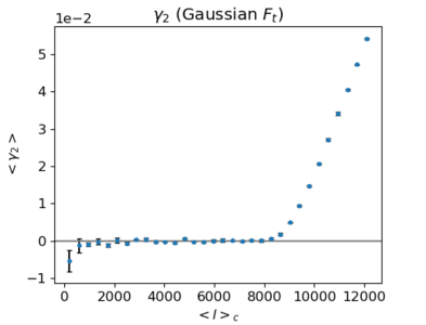
The plot above is the filtered kurtosis of Gaussian realizations of the CIB. It may be that the rising kurtosis at high [math]\displaystyle{ \ell }[/math] for the CIB without the brightest pixels can also be an 'NSIDE artifact'; I am planning to check this with a lower cut-off for the brightest galaxies. It does seem essential to leave out [math]\displaystyle{ \ell \gt 8000 }[/math] for the kurtosis in future analyses however.

-Expected reduced bispectrum, comparison with Poisson

Meanwhile, the expected [math]\displaystyle{ b_{\ell} }[/math] drops by 1~2 orders of magnitude, but the right plot remains flat at high [math]\displaystyle{ \ell }[/math].

In the right plot, the filtered skewness seems to match very well with the Poisson value at [math]\displaystyle{ \ell \gt 2000 }[/math], suggesting that the brightest pixels may not follow Poisson statistics very well.

The expected [math]\displaystyle{ b_{\ell} }[/math] is as such:

Original CIB: [math]\displaystyle{ b_{\ell} \approx 360Jy^3/sr }[/math]

CIB without the brightest galaxies: [math]\displaystyle{ b_{\ell} \approx 7.2Jy^3/sr }[/math]

-3rd moment

The 3rd moment, similar to the normalized skewness, starts at a similar value as the original CIB (note that the y-axis scales differ) but then drops and remains essentially flat.

Another thing to note is that for the CIB without the brightest galaxies, the 3rd moment, reduced bispectrum, and filtered skewness all show very similar trends, only on different magnitudes.

                 3rd Moment                        Expected [math]\displaystyle{  b_{\ell}  }[/math] calculated from sims                      Filtered skewness