May 21th, 2019 - New Plots with NSIDE 4096

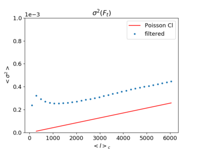
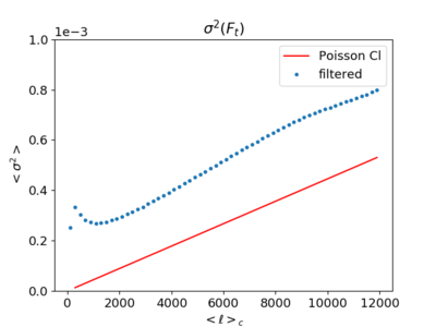
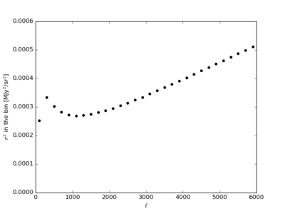
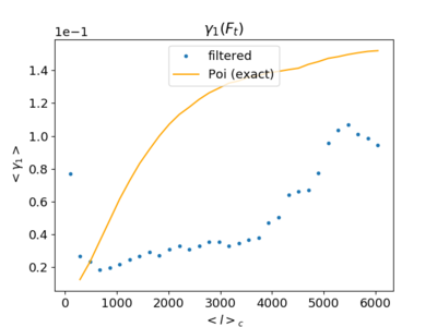
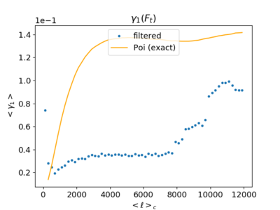
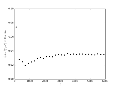
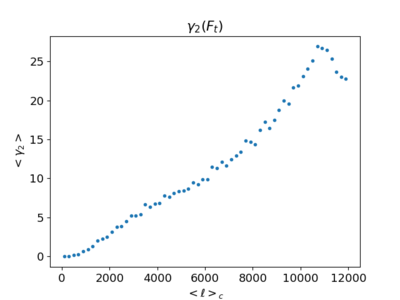
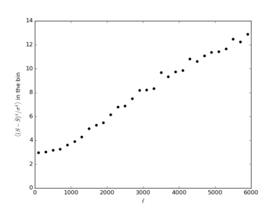
I have at last top-hat filtered the NSIDE = 4096 CIB map, so here I simply compare previous plots with NSIDE 2048 to the new ones. The left are the 2048 while the middle the 4096, and the right are Pavel's plots. For the filtering, I used 60 bands from [math]\displaystyle{ 0 \le \ell \le 12000 }[/math] with [math]\displaystyle{ \Delta \ell = 200 }[/math].

Previously, it was [math]\displaystyle{ 0 \le \ell \le 6144 }[/math] with [math]\displaystyle{ \Delta \ell = 192 }[/math].

In this post, I am referring the skewness and kurtosis to be the normalized skewness and excess kurtosis ([math]\displaystyle{ \lt \frac{(S - \bar{S})^3}{\sigma^3}\gt }[/math] and [math]\displaystyle{ \lt \frac{(S - \bar{S})^4}{\sigma^4}\gt -3 }[/math]), while the 3rd moment and 4th moment refer to the un-normalized skewness/kurtosis.

Filtered Variance (With the Poisson curve)

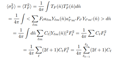
On the middle plot, the variance continues to increase as [math]\displaystyle{ \ell }[/math] increase, which makes sense considering the following expression and the fact that [math]\displaystyle{ C_{\ell} }[/math] does not decrease as rapidly at high [math]\displaystyle{ \ell }[/math].

Filtered Skewness (With the Poisson curve)

The skewness, contrary to the variance, does not continue increasing; it rather looks like only the x-axis has been replaced with numbers twice as large. This is a bit puzzling, as the approximation from a previous post (https://mocks.cita.utoronto.ca/index.php/May_6th,_2019_-_Calculating_the_Poisson_variance_and_skewness_(first_attempt)) gives: [math]\displaystyle{ S_3 \propto [(l_b - l_{b-1})^2 \frac{1}{\sqrt{3} \pi^3} \sum_{l = l_{b-1}}^{l_b} l ]b_{l,l,l} \propto (l_b - l_{b-1})^2 l^2 }[/math] which means that the skewness should at least be increasing since [math]\displaystyle{ b_l }[/math] should be nearly constant at high [math]\displaystyle{ \ell }[/math].

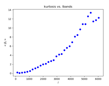
Filtered Kurtosis (note that my plot is offset on the y-axis by 3, which seems to be because Pavel used the kurtosis while I used the excess kurtosis)

The kurtosis behaves in a similar way to the variance; it continues on after [math]\displaystyle{ \ell \gt 6000 }[/math]. (The different y-axis label on the left plot is a different notation I used in past plots.)

Conclusion

The variance and kurtosis plots seem uneventful when the NSIDE increase, they just continue on in similar fashions as before. The skewness plot is puzzling however, I cannot think of a legitimate reason to explain why it behaves differently when NSIDE is increased; one difference that may be (but I doubt this) related is that the skewness is an odd function (odd power) while the variance and skewness are even functions.