May 6th, 2019 - Calculating the Poisson variance and skewness (incomplete)

I am looking into calculating the Poisson [math]\displaystyle{ C_\ell }[/math] and [math]\displaystyle{ b(\ell_1, \ell_2, \ell_3) }[/math] and using them to compare with the filtered variance and skewness from the simulations.

Power Spectrum and Filtered Variance

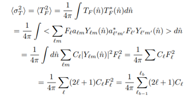
Relating [math]\displaystyle{ C_\ell }[/math] to the filtered variance is simple for the case of the top-hat filters:

with [math]\displaystyle{ \ell_{b-1} }[/math] and [math]\displaystyle{ \ell_b }[/math] being the start and end values of [math]\displaystyle{ \ell }[/math] and [math]\displaystyle{ F_{\ell} = 1 }[/math] within a band.

Reduced Bispectrum and Filtered Skewness

For the relation between [math]\displaystyle{ b(\ell_1, \ell_2, \ell_3) }[/math] and the filtered skewness, I am using the relations from Komatsu et al. 2000 (https://arxiv.org/pdf/astro-ph/0005036.pdf) and Bhattacharya et al. 2012 (https://iopscience.iop.org/article/10.1088/0004-637X/760/1/5/pdf) ([math]\displaystyle{ \ell \gt 500 }[/math] for the bottom equation) :

where [math]\displaystyle{ L = \ell_1 + \ell_2 + \ell_3 }[/math] and the Wigner-3j symbols vanish for odd [math]\displaystyle{ \ell }[/math].

With [math]\displaystyle{ W_{\ell} }[/math] being 1 for the top-hat filters,

[math]\displaystyle{ S_3 = \frac{1}{\pi^3} \sum_{2 \le l_1 l_2 l_3} (l_1 + \frac{1}{2})(l_2 + \frac{1}{2})(l_3 + \frac{1}{2}) \frac{(-1)^L}{\sqrt{(L(L-2l_1)(L-2l_2)(L-2l_3)}} b_{l_1 l_2 l_3} }[/math]

[math]\displaystyle{ \approx (l_b - l_{b-1})^2 \frac{1}{\sqrt{3} \pi^3} \sum_{l = l_{b-1}}^{l_b} \frac{(l + \frac{1}{2})^3}{l^2} b_{l,l,l} \approx [(l_b - l_{b-1})^2 \frac{1}{\sqrt{3} \pi^3} \sum_{l = l_{b-1}}^{l_b} l ]b_{l,l,l} }[/math]

where in the bottom line, I have used [math]\displaystyle{ \ell_1 \approx \ell_2 \approx \ell_3 \approx \ell }[/math] and the square term in the front arises due to the number of permutations (a rough approximation of it at least).

Poisson Power Spectrum and Reduced Bispectrum

For the Poisson power spectrum and reduced bispectrum, I am using the expressions we discussed before:

[math]\displaystyle{ C_\ell^{Poi} = \int dS s^2 \frac{dN}{dSd\Omega} }[/math]

and

[math]\displaystyle{ b_\ell^{Poi} = \int dS s^3 \frac{dN}{dSd\Omega} }[/math]

with [math]\displaystyle{ dN }[/math] being the number of galaxies within a flux bin ([math]\displaystyle{ dS }[/math]), and [math]\displaystyle{ d\Omega = 4\pi }[/math].

CIB Flux Histogram

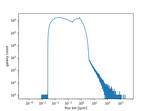
Using the CIB flux histogram George provided, this seems to be fairly simple.

However, the flux bins of the histogram is in [math]\displaystyle{ log_{10} }[/math], so using the size of the bins as [math]\displaystyle{ dS }[/math] may be inaccurate as the bin size begins as about [math]\displaystyle{ 10^{-8} }[/math] on the first index but increases to around [math]\displaystyle{ 10 }[/math] on the last index (a total of 10000 bins).

Power Spectrum / Filtered Variance Calculation

Starting with the power spectrum,

Taking the flux [math]\displaystyle{ s }[/math] to be the midpoints of each bin, and taking the Riemann sum: [math]\displaystyle{ C_\ell^{Poi} = \int dS s^2 \frac{dN}{dSd\Omega} \approx \sum_{i = 1}^{nbins} \Delta s \frac{N_i}{\Delta s} s_i^2 \frac{1}{d\Omega} = \sum N_i s_i ^2 \frac{1}{d\Omega} }[/math]

The value I obtained (using the calculations above) for the Poisson power spectrum is [math]\displaystyle{ C_\ell^{Poi} \approx 6.34 \times 10^7 Jy^2/sr }[/math], or [math]\displaystyle{ 6.34 \times 10^{-5} MJy^2/sr }[/math]. This is way too large compared to both the sims results ([math]\displaystyle{ 10^{-9} to 10^{-7} MJy^2/sr or 10^3 to 10^5 Jy^2/sr }[/math]) or the Planck 2013 XXX results for [math]\displaystyle{ \ell \gt 500, C_{\ell} \approx 10^3 }[/math] to [math]\displaystyle{ 10^4 Jy^2/sr }[/math] (Cosmic infrared background measurements and implications for star formation) (https://www.aanda.org/articles/aa/pdf/2014/11/aa22093-13.pdf).

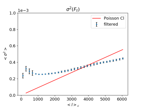
A plausible value for the Poisson power spectrum would be (obtained from back-tracking): [math]\displaystyle{ 3 \times 10^{-9} MJy^2 /sr (10^3 Jy^2/sr) }[/math]. which would give a plot as below:

Reduced Bispectrum / Filtered Skewness Calculation

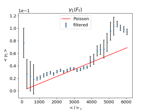
By calculating the Poisson reduced bispectrum in a similar way as above, I obtained the value: [math]\displaystyle{ 3.5 \times 10^9 Jy^3/sr (10^{-9}MJy^3/sr) }[/math], which is also drastically off from Planck values (which is on the order of [math]\displaystyle{ 10^3 Jy^3/sr }[/math] at [math]\displaystyle{ 200 \lt \ell \lt 600 }[/math]), but a plausible value calculated from the filtered skewness would be around [math]\displaystyle{ 5 \times 10^8 Jy^3/sr (10^{-10}MJy^3/sr) }[/math] which would give the plot below:

In Addition

I am also attempting other methods to calculate the Poisson [math]\displaystyle{ C_{\ell} }[/math] and [math]\displaystyle{ b_{\ell} }[/math], namely by setting:

[math]\displaystyle{ \frac{dN}{d\ln S} = s \frac{dN}{dS} }[/math] or [math]\displaystyle{ \log(dS) }[/math] for the log bins, but I am not entirely sure how this can be done (or even if these methods would accurately describe the log bins).

Another method I have been working on is to bin the flux histogram linearly; this has proven to be harder than I imagined as the number of log bins corresponding to one linear bin would vary drastically (much smaller than 1 to much larger than 1) as the flux increases. Setting the number of linear bins as [math]\displaystyle{ 10^6 }[/math] took too long for the computer to calculate, while setting the number to [math]\displaystyle{ 10^4 }[/math] did not generate an accurate version of the original flux histogram (the very 1st linear bin in this case would contain 5000 original log bins).

I also have not accounted for the fact that the flux bins in the original histogram is given in Jy/sr, but I doubt this would explain the multiple orders of magnitudes of differences I have been facing.