Nov 4, 2019 - Looking at factor 3 in bispectra

Motivation

When Jason calculates the equilateral bispectrum using our technique (we filter a map to include only a range of ell, we cube it, we calculate the mean), he gets bispectrum that is too high when compared with the Planck experimental values. In all 217 GHz, 353 GHz, 545 GHz, by about a factor of three. We are trying to understand what is going on.

Cell

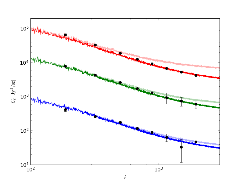
As a first thing we try reproducing Planck Cell. They are using bins with ell boundaries [145, 229, 411, 592, 774, 1006, 1308, 1701, 2211]. The Planck data are given in Table D2 of https://arxiv.org/pdf/1309.0382.pdf and are represented by the scatter points on the plot (most are to small to be visible):

The maps George produces are in MJy/sr. We calculate the variance of the filtered map, then convert it to the power spectrum assuming constant Cell. Those are the solid lines and we see that 545 GHz is not matching well.

We can also just calculate the C_ell directly, gives consistent result (the ones with alpha):

Could be related to cuts, which we do next. George claims about cuts that "You can feel free to use the Planck values of [350, 225, 315, 350, 710] mJy for [143, 217, 353, 545, and 857] GHz ...". After applying these cuts, we get the dark curves above, that match Planck data at high ell better.

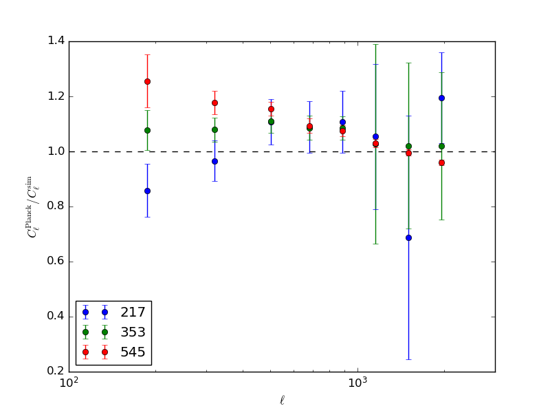
To better evaluate the match after making the flux cuts, we look at the ratio

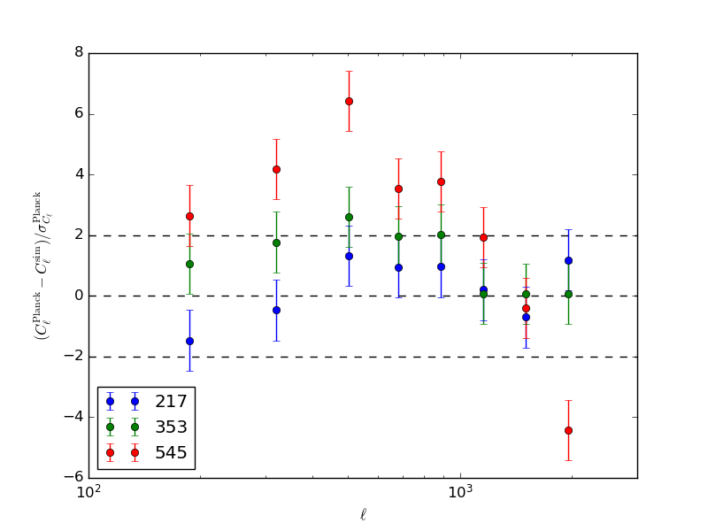
We see a match at the 10-20% level. There is some bias visible in the higher two frequencies, the following plot shows the significance determined by the Planck error bars (simulated Cell are nicely smoothed).

Bispectra theory

In our previous post from May 20, 2019 we use the Komatsu, Spergel definitions

[math]\displaystyle{ \langle a_{\ell_1m_1} a_{\ell_2m_2} a_{\ell_3m_3} \rangle = \sqrt{\frac{(2\ell_1+1)(2\ell_2+1)(2\ell_3+1)}{4\pi}} \begin{pmatrix} \ell_1 & \ell_2 & \ell_3\\ 0 & 0 & 0 \end{pmatrix} \begin{pmatrix} \ell_1 & \ell_2 & \ell_3\\ m_1 & m_2 & m_3 \end{pmatrix} b_{\ell_1 \ell_2 \ell_3} }[/math]

The Planck papers cite values for [math]\displaystyle{ b_{\ell_1 \ell_2 \ell_3} }[/math], we checked their definitions.

Komatsu, Spergel paper then relate this to skewness

[math]\displaystyle{ S_3 = \frac{1}{4\pi} \sum_{\ell_1 \ell_2 \ell_3} \frac{(2\ell_1+1)(2\ell_2+1)(2\ell_3+1)}{4\pi} \begin{pmatrix} \ell_1 & \ell_2 & \ell_3\\ 0 & 0 & 0 \end{pmatrix}^2 W_{\ell_1}W_{\ell_2}W_{\ell_3} b_{\ell_1\ell_2\ell_3} , }[/math]

we checked this relation again. The most tricky part is

[math]\displaystyle{ 1 = \sum_{m_1,m_2,m_3} \begin{pmatrix} \ell_1 & \ell_2 & \ell_3\\ m_1 & m_2 & m_3 \end{pmatrix}^2 }[/math]

Let's look now again at what we are trying to do - we filter the map, take the third power and then average over the pixels. This leads to

[math]\displaystyle{ \begin{array}{lcl} \langle M_F^3 \rangle &=& \frac{1}{N_\mathrm{pix}} \sum_\mathrm{pix} \sum_{\ell,m,\ell',m',\ell'',m''} a_{\ell m} a_{\ell' m'} a_{\ell'' m''} Y_{\ell m} (\theta_i) Y_{\ell' m'} (\theta_i) Y_{\ell'' m''} (\theta_i) \\&=& \frac{1}{4\pi}\times \frac{4\pi}{N_\mathrm{pix}} \sum_\mathrm{pix} \sum_{\ell,m,\ell',m',\ell'',m''} a_{\ell m} a_{\ell' m'} a_{\ell'' m''} Y_{\ell m} (\theta_i) Y_{\ell' m'} (\theta_i) Y_{\ell'' m''} (\theta_i) \\&=& \frac{1}{4\pi} \sum_{\ell,m,\ell',m',\ell'',m''} a_{\ell m} a_{\ell' m'} a_{\ell'' m''} \sum_\mathrm{pix} \frac{4\pi}{N_\mathrm{pix}} Y_{\ell m} (\theta_i) Y_{\ell' m'} (\theta_i) Y_{\ell'' m''} (\theta_i) \\&\approx& \frac{1}{4\pi} \sum_{\ell,m,\ell',m',\ell'',m''} a_{\ell m} a_{\ell' m'} a_{\ell'' m''} \int d^2 \theta Y_{\ell m} (\theta) Y_{\ell' m'} (\theta) Y_{\ell'' m''} (\theta) \\&\rightarrow& S_3 \end{array} }[/math]

The first line is just the definition, the next one is trivial, then we reorder the terms to a more suggestive form, then we use the fact that the sum over the pixels approximates the Gaunt integral and finally take the expectation value over the cosmic realizations.

Planck bispectra data

Planck quotes values of various bispectra [math]\displaystyle{ b_{\ell \ell' \ell''} }[/math], in the units of Jy^3/sr. Note that some of the values in D3 in the Planck XXX paper are wrong in terms of the orders of magnitude; should be using the data from Lacasa email. They use bands with ell boundaries [129, 257, 385, 513, 641, 769].

Assuming constant bispectrum b in the band, we can write

[math]\displaystyle{ \langle M_\ell^3 \rangle = b_{\ell \ell \ell} \sum_{\ell_1 \ell_2 \ell_3} \frac{(2\ell_1+1)(2\ell_2+1)(2\ell_3+1)}{16\pi^2} \begin{pmatrix} \ell_1 & \ell_2 & \ell_3\\ 0 & 0 & 0 \end{pmatrix}^2 \approx b_{\ell \ell \ell} \frac{\ell}{\sqrt{3}\pi^3} \times \frac{(\Delta \ell)^3}{2} , }[/math] where the approximate expression was derived earlier.

For the Planck configuration, the sum evaluates to [3.97412e6, 6.3601e6, 8.82929e6, 1.13136e7, 1.38037e7] and is well approximated by the formula above (5% error in the first bin, 2% in the second and dropping).

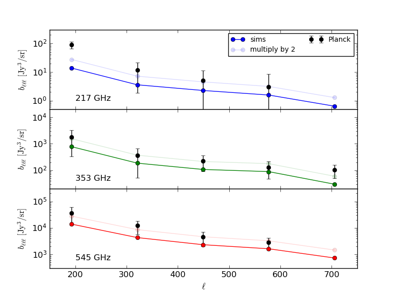
Calculating [math]\displaystyle{ \langle M_\ell^3 \rangle }[/math] from our sims and using the numerical factors above to recover the bispectrum, we get the following (the weak lines correspond to double the result from simulations):

This is using the flux cuts listed above. Looks like there might be a factor 2 off somewhere.

Looked at the estimator used by Planck, described in https://arxiv.org/pdf/1107.2251.pdf . It looks like they are formally doing exactly the same thing we are (their Eqn 7, 8): filter the map, build a third power of the filtered maps and take a suitably normalized mean (they express the mean as an integral over the sphere in their formulas, but the algebra seems to be identical to what we are doing).

We also checked how much do the bispectra change when we alter the flux cutoff. As a limiting step, we do not cutting on flux and we get the following:

So in principle, the discrepancy we are seeing might be somewhat related to the flux cutoff.