Oct 17th, 2019 - Discrepancies between Planck, SPT, and 'Sims' Bispectra?

Since Professor Bond suggested there may be a factor of [math]\displaystyle{  \pi  }[/math] difference between our bispectrum estimator and Planck's (see plots above), I took a look at the Planck XXX (2013, CIB) paper to see how they calculated the bispectra. Unfortunately, I cannot find a reason why such a factor should arise. So I also took a look at the SPT data at 220GHz (the "Crawford plot," as well as their released data) to see if I could find any clues. But more questions arose when I did this. 

In short, the Planck data (at low [math]\displaystyle{  \ell  }[/math]) seems to be about 3 times higher than 'sims' values, while the Crawford data (at high [math]\displaystyle{  \ell  }[/math]) seems to be around [math]\displaystyle{  \sqrt{4\pi}  }[/math] ~ [math]\displaystyle{  4\pi  }[/math] times lower than 'sims' values depending on whether or not the [math]\displaystyle{  \sqrt{4\pi}  }[/math] (https://mocks.cita.utoronto.ca/index.php/Aug_18th,_2019_-_CIB_Bispectrum:_Comparison_With_Crawford_Plot_(217GHz,_Poisson_Part)) I mentioned in a previous post is necessary.  Why is 'sims' smaller than Planck values but higher than SPT??  (Perhaps because Planck gives us data at low [math]\displaystyle{  \ell  }[/math] and SPT gives us data at high [math]\displaystyle{  \ell  }[/math], there may be no correlation between the two ranges?)

Planck's Bispectrum Estimator

First, I present how Planck XXX (2013) (https://www.aanda.org/articles/aa/pdf/2014/11/aa22093-13.pdf) calculated their bispectra coefficients. 

 

The Planck Paper points to Lacasa et al. (2012) (https://academic.oup.com/mnras/article/421/3/1982/1075516), where Eq.(5) is simply another expression that can be obtained by combining Eq. (2), (3), (6) of Komatsu & Spergel (2000) (https://arxiv.org/pdf/astro-ph/0005036.pdf) shown below:  

Since the [math]\displaystyle{  N_{\Delta}  }[/math] factor in Eq.(8) of Lacasa et al. is simply the number of configurations within a bin, our bispectrum estimator should be calculating the same thing without any [math]\displaystyle{  \pi  }[/math] factors. The way we define our bispectrum estimator is given in (https://mocks.cita.utoronto.ca/index.php/May_20,_2019_-_Bispectra_of_the_Poisson_field) (Pavel's post when he was checking my calculations), and uses Komatsu & Spergel's definition. 

SPT Comparison

I previously put up a post (https://mocks.cita.utoronto.ca/index.php/Aug_18th,_2019_-_CIB_Bispectrum:_Comparison_With_Crawford_Plot_(217GHz,_Poisson_Part)) containing a plot comparing our 'sims' data with Crawford et al. (2014) (https://iopscience.iop.org/article/10.1088/0004-637X/784/2/143/pdf)'s plot.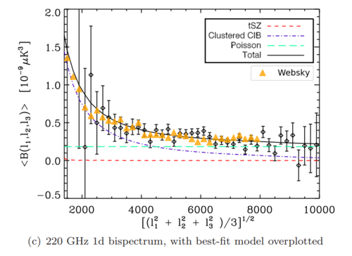 

The above plot was made by converting the old 'sims' values to [math]\displaystyle{  \mu K^3  }[/math] simply dividing the 3rd power of Jy/sr -> microK conversion factor (https://mocks.cita.utoronto.ca/index.php/File:Conversion_factors.png) and dividing again by [math]\displaystyle{  \sqrt{4\pi}  }[/math] on the grounds of the dimensional analysis given in that post. 

There are two issues: 

1) I tried reproducing the Crawford plot with the data they have online (https://pole.uchicago.edu/public/data/crawford13/index.html), but it does not work when I take the average bispectra values within a bin and divide by the number of configurations. The plots below are: Reproduction Attempt (left), plot of Equilateral configurations only (right)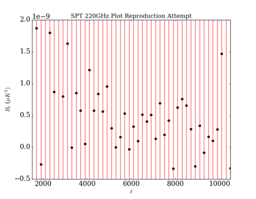

 

While the shape of the first plot somewhat resembles the plot from the paper, they are clearly different. I have no idea why the error bars are so large (I used the square root of the covariance matrix as usual), nor do I understand how there can be negative values. The weighting definitely has some effect in causing the difference between the plot in the paper and my plot (where all the weights are 1); this was the reason I was thinking of e-mailing Professor Crawford. 
 
The second plot shows us that we cannot compare strictly the equilateral data from SPT; I do not understand why the values fluctuate so much 

Here I have a question: Does it make sense to compare our equilateral bispectrum values with the SPT plot when their plot contains a weighted average of all the configurations? (I have noticed that the equilateral values are usually substantially larger than other values.) 

If it is, then we may benefit by asking Professor Crawford about the weights; then we could calculate the values for low [math]\displaystyle{  \ell  }[/math] as well (not shown in the plots) which we could compare with the Planck and 'sims' data. 

2) I compared the values calculated from the new map and the old map. However, there's a huge discrepancy at high [math]\displaystyle{  \ell  }[/math]:

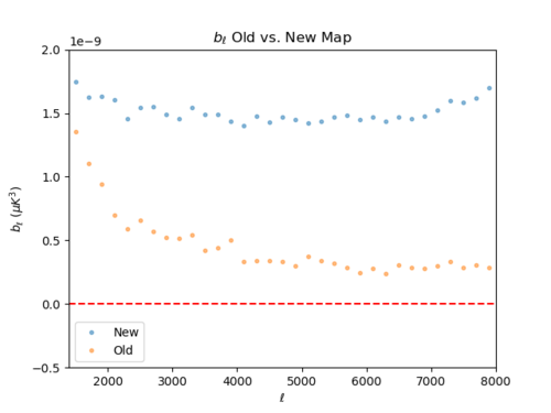
The only reason I could think why is because the masking flux cut was different between the two. The new map's flux cut was 400mJy as George said. The old map's was much lower (because back then I had removed the same number of bright pixels from each of the maps). I am thinking that the flux cut may have to be lowered for 217GHz relating to the frequency since the shape of the old map's values (resembling a 1/x curve) matches the SPT plot much better.