May 15th, 2019 - Flux Re-normalization & Poisson variance/skewness

Thanks to the discussion we had last week, I was able to re-normalize the CIB flux histogram and calculate the Poisson variance and skewness; the values now seem reasonable.

Re-normalization

Taking a look at the flux histogram from the previous post (https://mocks.cita.utoronto.ca/index.php/May_8th,_2019_-_Some_analysis_on_the_sims_map_and_the_expected_Poisson_bispectrum), we agreed that the total flux calculated from the histogram should match the value calculated from the map:

[math]\displaystyle{ A [\sum_{i} N_i(S_i) * S_i] = \mu_{\text{map}} * N_{\text{pix}} * \frac{4\pi}{N_{\text{pix}}} = 4\pi \mu_{\text{map}} }[/math]

[math]\displaystyle{ S_i }[/math] is the (mean of) flux of bin 'i', [math]\displaystyle{ N_i }[/math] the number of galaxies in flux bin 'i', [math]\displaystyle{ \mu_{\text{map}} }[/math] the mean flux value in the map (0.333 MJy/sr), and [math]\displaystyle{ N_{\text{pix}} }[/math] the number of pixels in the map and [math]\displaystyle{ A }[/math] the factor of re-normalization.

Using the expression above, the factor [math]\displaystyle{ A }[/math] is calculated to be about 0.017355, which is close, but smaller than the factor I had estimated in the previous post (1/40).

The re-normalized flux histogram is given below.

The 'peak' (the odd vertex) is now at around S = 4mJy.

Comparison with Reference Values

To check the plausibility of the histogram above, I plotted [math]\displaystyle{ S^{2.5} \frac{dN}{dS} }[/math] (which I will refer to as 'y') against [math]\displaystyle{ S }[/math] and compared it to the reference plot(s) also from the previous post.

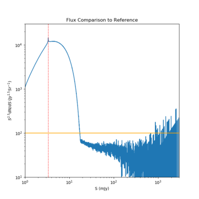
The location of the peak in the sims plot (red dotted line) is at 3.63 mJy which is quite similar to the reference plot. The peak value is similar as well at around [math]\displaystyle{ 10^4 }[/math] (note that the reference plot's y-axis is in log). Although the negative slope for the sims plot is steeper compared to the reference plot, the y values seem to flatten out at higher S values. The ragged y-values towards the right in the sims plot is due to the much wider (log) bins at high S. The reference plot also displays a plateau at high S, but at higher y-values ([math]\displaystyle{ \gt 10^2 }[/math]) compared to the sims plot; these higher values are due the contribution from strong-lensed galaxies, their fluxes becoming 10 or even 100 times larger than their original fluxes (Alex explained to me about this).

In short, the sims plot looks close enough to the reference plot that the subsequent Poisson calculations can be trusted.

Poisson Power Spectrum and the Filtered Variance Plot

Using the expression for the power spectrum in the Poisson regime as before (and the re-normalized flux histogram), [math]\displaystyle{ C_\ell^{Poi} = \int dS s^2 \frac{dN}{dSd\Omega} }[/math] the Poisson power spectrum is calculated to be around [math]\displaystyle{ 1.4 \times 10^3 Jy^2/sr }[/math]. A comparison between the power spectra obtained in different ways (Planck, sims with different NSIDEs, Poisson) is given below.

The power spectrum from even the NSIDE = 4096 sims does not exactly match the Poisson power spectrum at high [math]\displaystyle{ \ell }[/math], but [math]\displaystyle{ \ell }[/math] does not go high enough for any of the sims to show a completely flat regime. At [math]\displaystyle{ \ell \approx 10000 }[/math], the sims power spectrum is about 2 times larger than the Poisson.

Using the power spectrum value above, I also plotted how the filtered variance would look like in the Poisson limit.

Again, the magnitude is off (by 2 ~ 10 times) but the slope is nearly the same judging from the fact that the two curves are almost parallel (the slopes matching may not be significant physically).

A Blunder in Previous Skewness/Bispectrum Calculations, But Has It Been Resolved?

Before moving onto the 3-point function, I must point out what had been causing the multiple orders of magnitude - offset between the Poisson reduced bispectrum and the sims' reduced bispectrum. In a previous post (https://mocks.cita.utoronto.ca/index.php/May_6th,_2019_-_Calculating_the_Poisson_variance_and_skewness_(first_attempt)), I derived the equation (at [math]\displaystyle{ \ell \gt 500 }[/math])

[math]\displaystyle{ S_3 = \frac{1}{\pi^3} \sum_{2 \le l_1 l_2 l_3} (l_1 + \frac{1}{2})(l_2 + \frac{1}{2})(l_3 + \frac{1}{2}) \frac{(-1)^L}{\sqrt{(L(L-2l_1)(L-2l_2)(L-2l_3)}} b_{l_1 l_2 l_3} }[/math]

where I assumed that [math]\displaystyle{ S_3 }[/math] is the skewness value within each [math]\displaystyle{ \ell }[/math]-band. However, the skewness calculated by 'scipy.stats.skew' is defined differently from the reference paper I had consulted.

'Scipy's definition'

[math]\displaystyle{ S_3 = \lt (\frac{ (X -\mu) }{\sigma})^3\gt }[/math]

'Komatsu et al. 2000'

[math]\displaystyle{ S_3 = \lt (\frac{ \Delta T(\hat n) }{T})^3\gt }[/math]

So in order to relate the filtered skewness to [math]\displaystyle{ b_{l_1 l_2 l_3} }[/math], we must account for the [math]\displaystyle{ \sigma }[/math] and the [math]\displaystyle{ T }[/math] (mean flux in the map in MJy/sr) factors: [math]\displaystyle{ S_3 = \frac{T^3}{\sigma^3} \frac{1}{\pi^3} \sum_{2 \le l_1 l_2 l_3} (l_1 + \frac{1}{2})(l_2 + \frac{1}{2})(l_3 + \frac{1}{2}) \frac{(-1)^L}{\sqrt{(L(L-2l_1)(L-2l_2)(L-2l_3)}} b_{l_1 l_2 l_3} }[/math]

However, now the units on the left-hand side (LHS) and right-hand side(RHS) of the equation do not match. The LHS is dimensionless while the RHS has a unit of [math]\displaystyle{ Jy^3/sr }[/math], since the [math]\displaystyle{ \sigma^3 }[/math] and the [math]\displaystyle{ T^3 }[/math] cancel each others' units out.

For subsequent calculations, I have left out the [math]\displaystyle{ T^3 }[/math] for now, so that the 'Jy' (or 'MJy') factors in the numerator and denominator cancel out on the RHS (there may be extra factors of [math]\displaystyle{ 4\pi }[/math] left on the RHS because of the 'sr' factors as well).

Poisson (Reduced) Bipectrum

The Poisson bispectrum was calculated with the expression [math]\displaystyle{ b_\ell^{Poi} = \int dS s^3 \frac{dN}{dSd\Omega} }[/math] as before. Its value is: [math]\displaystyle{ 359 Jy^3/sr }[/math].

Below are the plots of the Poisson bispectrum calculated with the filtered skewness. On the left is the expected reduced bispectrum obtained from the filtered skewness (log scale), while the right is its comparison to the Poisson bispectrum.

The mean bispectrum at high [math]\displaystyle{ \ell }[/math] for the sims is just larger than the Poisson value at around [math]\displaystyle{ 420 Jy^3/sr }[/math]

I was also intending to compare the sims and Poisson bispectrum values to the SPT value (in the plot above), but so far I have been unsuccessful with the conversion between [math]\displaystyle{ \mu K^3 }[/math] and [math]\displaystyle{ Jy/sr }[/math].

Poisson Filtered Skewness

From the relation obtained from a previous post, [math]\displaystyle{ S_3 = \frac{1}{\pi^3} \sum_{2 \le l_1 l_2 l_3} (l_1 + \frac{1}{2})(l_2 + \frac{1}{2})(l_3 + \frac{1}{2}) \frac{(-1)^L}{\sqrt{(L(L-2l_1)(L-2l_2)(L-2l_3)}} b_{l_1 l_2 l_3} }[/math]

[math]\displaystyle{ \approx (l_b - l_{b-1})^2 \frac{1}{\sqrt{3} \pi^3} \sum_{l = l_{b-1}}^{l_b} \frac{(l + \frac{1}{2})^3}{l^2} b_{l,l,l} \approx [(l_b - l_{b-1})^2 \frac{1}{\sqrt{3} \pi^3} \sum_{l = l_{b-1}}^{l_b} l ]b_{l,l,l} }[/math]

I also calculated the filtered skewness in the Poisson limit.

The plot above shows the Poisson filtered skewness to be somewhat larger than the sims filtered skewness; both values increase as [math]\displaystyle{ \ell }[/math] increase, but the manners they increase are different.

The plot above compares Poisson filtered skewness curves calculated using the approximated sum (which I was doing previously, https://mocks.cita.utoronto.ca/index.php/May_6th,_2019_-_Calculating_the_Poisson_variance_and_skewness_(first_attempt)) and the exact sum. For the exact sum, I did not consider any configurations where [math]\displaystyle{ L = l_1 + l_2 + l_3 }[/math] is odd (meaning that I divided by 2), and calculated each component within the sum for every configuration of the [math]\displaystyle{ \ell }[/math]'s within the band. (All [math]\displaystyle{ \ell }[/math] values except for the first band satisfies the triangle inequality)

The approximation and the exact sum differs by a factor of (roughly) 3, about 1.5 if I had simply divided the approximated sum by 2 (disregarding the odd [math]\displaystyle{ L }[/math]

3rd Moment or Skewness?

In this section, I am displaying the filtered skewness/3rd-moment plots (sims). The left plot is the filtered skewness vs. [math]\displaystyle{ \ell }[/math], while the right plot is the filtered 3rd-Moment vs. [math]\displaystyle{ \ell }[/math], which was obtained by multiplying [math]\displaystyle{ \sigma^3 }[/math] to the former plot.

The values of the y-axes between the two plots vary by several orders of magnitude as the variance is much smaller than unity. Their shapes however, are similar. For physical interpretation, it seems more reasonable to use the right plot (3rd moment), since it is directly relevant to the bispectrum (as seen in the equation from the previous sections), but there seems to be little difference in their trends (how they behave as a function of [math]\displaystyle{ \ell }[/math]).