May 8th, 2019 - Some analysis on the sims map and the expected Poisson bispectrum

I have compared some reference values (the power spectrum and mean intensity) with the values from the sims CIB map, and probed more into the expected Poisson power spectrum and reduced bispectrum.

Comparison to Reference Values

Power Spectrum (NSIDE = 2048, NSIDE =4096, and Planck 2013 XXX)

As expected, the power spectra of the 3 cases match very well.

The mean of the sims map, regardless of the NSIDE is around 0.333 MJy/sr (although I had thought there was a dependency between the NSIDE and the mean flux, this turned out to be false). In a very recent paper (which appeared about a week ago) by Odegard et al. (2019) (https://arxiv.org/pdf/1904.11556.pdf), the mean CIB intensity at 545GHz is listed as 0.371±0.018 MJy/sr, so the difference between the two values is about 10%.

The fact that the mean intensity of the map does not depend on NSIDE implies that the total flux calculated from the map and histogram may not necessarily match.

Discrepancy between the Poisson reduced bispectrum and Planck's measured bispectrum?

Using the equations from the previous post (https://mocks.cita.utoronto.ca/index.php/May_6th,_2019_-_Calculating_the_Poisson_variance_and_skewness_(incomplete) ), I calculated the expected [math]\displaystyle{ b_l }[/math] in the Poisson limit using the filtered skewness values (with 32 bands). Below are the [math]\displaystyle{ b_\ell }[/math] vs. [math]\displaystyle{ \ell }[/math] plots.

i) log y-axis

ii) linear y-axis (leaving out the first three values)

As seen above, [math]\displaystyle{ b_l }[/math] fluctuates about its mean when [math]\displaystyle{ \ell }[/math] is high enough.

However, the values are several orders of magnitudes larger than Planck's measured values (for strictly the equilateral component of [math]\displaystyle{ b_l }[/math]), which is puzzling.

Normalization factor of the flux histogram

The question now, is the normalization factor for the x-axis of the flux histogram. By comparing the location of the 'peak' of the flux histogram George provided, and the one Alex mentioned in a recent e-mail (https://www.cita.utoronto.ca/~engelen/plots/bethermin.png),

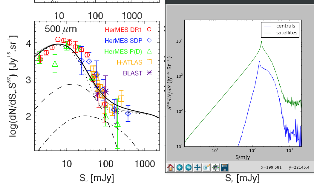
we can see that the location of the peak between the two histograms match, with the peak being at around 200mJy. (The normalization factor in this case was 1, instead of 3.7 (which George had originally put))

However, the Poisson [math]\displaystyle{ C_{\ell} }[/math] and [math]\displaystyle{ b_l }[/math] values in this case are: [math]\displaystyle{ 4.63 \times 10^6 Jy^2 /sr }[/math] and [math]\displaystyle{ 6.87 \times 10^7 Jy^3 /sr }[/math] respectively; still way too large.

Backtracking from the desirable [math]\displaystyle{ C_{\ell} }[/math] and [math]\displaystyle{ b_l }[/math] values ([math]\displaystyle{ 2.9 \times 10^3 Jy^2 /sr }[/math] and [math]\displaystyle{ 1.1 \times 10^3 Jy^3 /sr }[/math] (both similar to Planck values)), the normalization factor was 1/40. The flux histogram in this case is as below.

Now the flux values seem too low however.

Contribution to the Poisson [math]\displaystyle{ C_{\ell} }[/math] and [math]\displaystyle{ b_l }[/math] by flux

The two plots below describe how much each flux value contributes to the total [math]\displaystyle{ C_{\ell} }[/math] and [math]\displaystyle{ b_l }[/math]. (normalization factor: 1)

It is evident that nearly all of the contribution comes from fluxes larger than the location of the peak for the bispectrum (over 99.5%), while for the power spectrum, most (80%) of the contribution comes from fluxes larger than the location of the peak.